| << Previous | Contents | Next >> |
Based on the concepts described in Chapters 1-3, Chapter 4 begins examining how an Asset Sustainability Index could be built using existing U.S. transportation agency data. The index as proposed in this report is a composite of pavement, bridge and maintenance condition data. This chapter begins the analysis by examining the pavement component of the index, which would be a Pavement Sustainability Ratio. When that ratio is combined with the Bridge Sustainability Ratio and the Maintenance Sustainability Ratio, they would form the Asset Sustainability Index as proposed. This example uses pavement condition and expenditure data from the Ohio, Utah and Minnesota Departments of Transportation.
The Ohio Department of Transportation (ODOT) produces annual and multi-year reports that illustrate past, current and projected future pavement conditions. The long timeframe of the Ohio DOT reporting is intended to complement its long-standing policy of placing infrastructure preservation as the central focus of its long-term budgeting. Catch phrases for this emphasis have changed over the years with such terms as sustaining a "steady state" of acceptable infrastructure conditions to a "fix it first" approach. The policy approach has been supported by a reporting process that keeps the agency focused on ensuring that its capital budgeting process, its project-selection decisions and its maintenance practices work in concert to achieve stable, long-term infrastructure conditions within the constraints of available revenue.
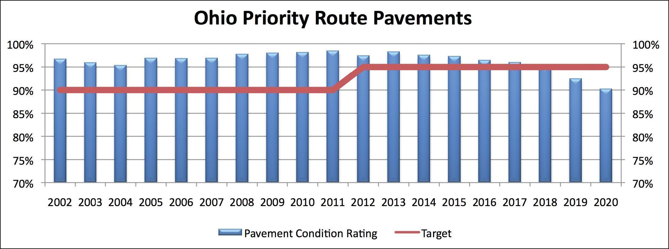
Figure 17: Conditions on Ohio's "priority system".
Inherent in the ODOT infrastructure-management process is a long planning horizon. As seen in Figure 17 above, the agency looks at a nearly 20-year timeframe. The past years provide a trend line of investment levels and resulting infrastructure conditions that yield a solid analytical baseline for future forecasts. By extrapolating from a long trend line, the agency builds confidence in its pavement deterioration curves and other inputs for its forecasts of future performance. By looking at least a decade into the future for many of its major system elements such as bridges and Priority System pavements, it keeps the agency focused upon substantive planning to ensure steady, long-term conditions. As seen in Figures 17 and 18, the agency has raised the target for Priority System pavement conditions from 90 percent acceptable to 95 percent.
Figure 18: Ohio pavement conditions over 30 years.
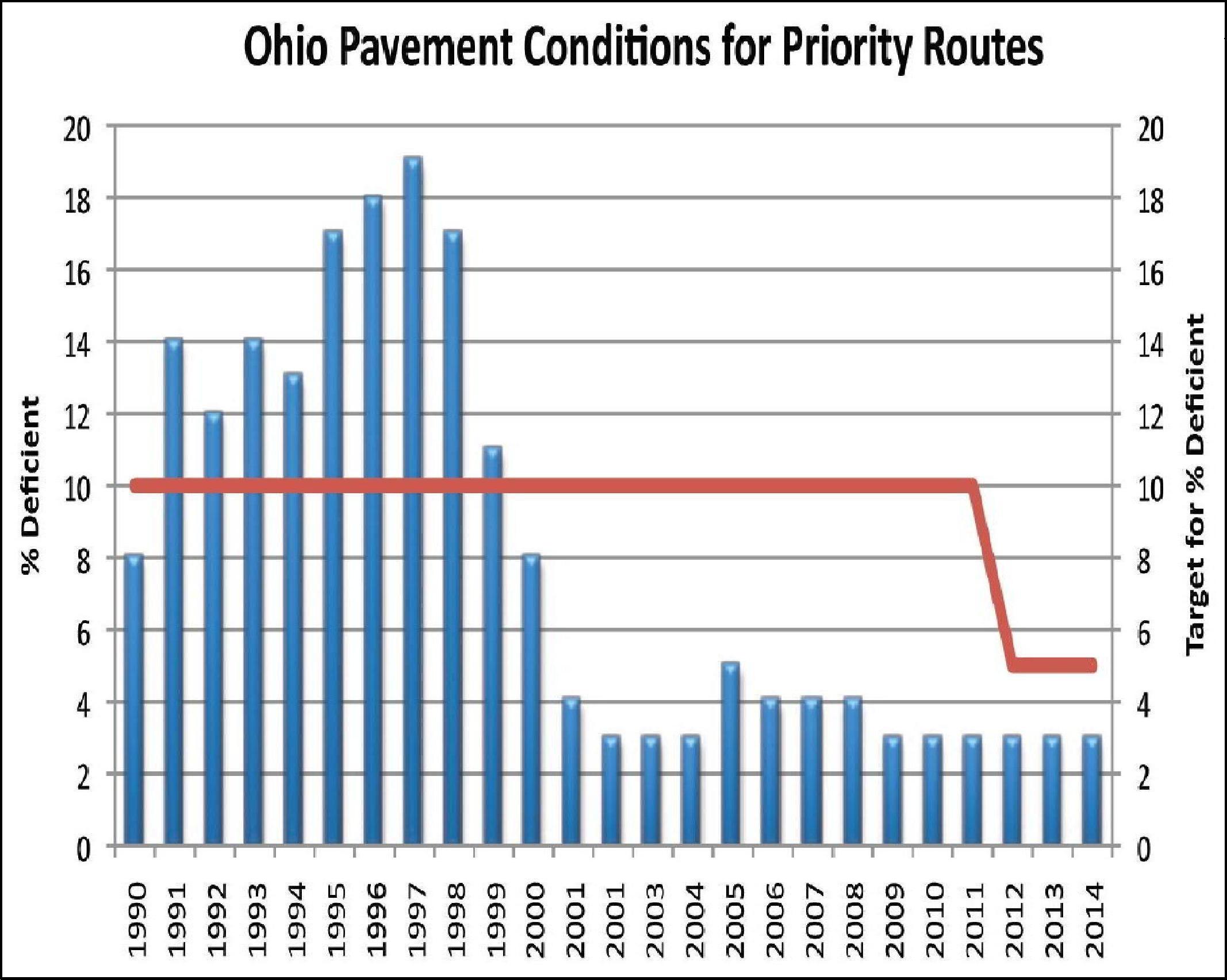
As seen in Figures 17 and 18, the agency has steadily surpassed its system condition goals for its Priority System. The Priority System in Ohio is similar to the National Highway System and it includes the Interstate Highway System and most multi-lane, divided routes. It consists of approximately 26 percent of the State's lane miles but handles 59 percent of the total vehicle miles of travel and 77 percent of the truck travel.[6] The State uses a Pavement Condition Rating (PCR) in addition to the International Roughness Index (IRI). The PCR is derived from an extensive visual survey of every route annually. The PCR is collected by a central crew of raters to ensure consistency. They measure more than 20 distresses including several that are indicative of structural pavement distresses such as reflective cracking, alligator cracking, pumping on concrete or composite pavements or broken slabs in concrete or composite pavements. The State also has compiled a construction history for every major pavement section, and it has a year-by-year history of past treatments and rates of PCR change by segment. This extensive history allows the department to forecast future conditions based upon scheduled treatments and each pavement's deterioration curve. The department has been stressing Asset Management for the past decade and that has contributed to substantial pavement condition improvements. In the mid-1990s, nearly 20 percent of the Priority System lane miles were below the acceptable PCR threshold of 65 and had substantial rates of annual degradation. As seen in Figure 18 above, the high deficiency volumes of the 1990s were addressed and system conditions have consistently surpassed the State's targets. The forecasted increase in deficiencies in the years after 2018 are largely, but not wholly, attributable to the State's forecasting methods. It forecasts conditions based upon the treatments programmed in the Statewide Transportation Improvement Program (STIP) as reported in the department's project-management system called Ellis. Because projects are not programmed yet for the later years, the Ellis program applies a deterioration curve to each pavement but does not yet capture the expected pavement treatments.
| Ohio Pavement Expenditures and Condition Results (Actual and Forecast) | ||||||||||||
|---|---|---|---|---|---|---|---|---|---|---|---|---|
| 2005 | 2006 | 2007 | 2008 | 2009 | 2010 | 2011 | 2012 | 2013 | 2014 | 2015 | Total | |
| General System Two-Lane Pavements | $93 | $93 | $108 | $113 | $179 | $186 | $147 | $149 | $151 | $152 | $154 | |
| Percent Acceptable | 98% | 97% | 97% | 97% | ||||||||
| Priority System Routine Maintenance | $179 | $179 | $217 | $228 | $192 | $199 | $143 | $145 | $146 | $148 | $149 | |
| Percent Acceptable | 0.96 | 0.97 | 0.97 | 0.97 | ||||||||
| Priority System Rehab and Replacement | $150 | $192 | $150 | $150 | $150 | $150 | $172 | $173 | $175 | $176 | $178 | |
| Paving State Routes in Cities | $35 | $35 | $35 | $35 | $35 | $35 | $35 | $35 | $35 | $35 | $35 | |
| Percent Acceptable | 96% | 95% | 90% | 90% | ||||||||
| Total Pavement Program Budgeted | $457 | $499 | $510 | $526 | $556 | $570 | $497 | $502 | $507 | $511 | $516 | $4,185 |
| Projected Shortfall for Pavement Program | -$139 | -$152 | -$166 | -$182 | -$198 | -$837 | ||||||
| Source: Amended ODOT 2006-2007 Business Plan | ||||||||||||
ODOT reports expenditure levels in a fashion similar to that required by GASB, by some of the international financial reporting processes and similar to what is envisioned for the Asset Sustainability Index. Although the details of the financial expenditure processes have changed over the years, the basic concept has been used for more than a decade. As seen above in Table 12 from the Department's amended 2006-2007 Business Plan, pavement expenditures were to rise from $457 million in 2005 to $516 million in 2015. The department manages its pavements in three systems, Priority, General and Urban. The Priority System already has been described, while the General System is basically the two-lane system outside of city limits, which in the "Home Rule" State of Ohio is the DOT's responsibility. The Urban System is basically State and U.S. routes within cities, which in Ohio are a shared responsibility between the State and local governments. As seen in the Table 12, the percentage of acceptable forecasted pavement conditions for the three systems range from a high of 98 percent for the Priority System in 2008 to a low of 90 percent for the Urban System by 2015. The targets for PCR conditions on the General and Urban Systems in 2006 were a PCR of 55.
Table 12 also shows a forecasted financial shortfall in needed pavement investment starting in 2011 and continuing through 2015. In the 2006 scenario, ODOT was forecasting that within five years it would experience a shortfall starting at $139 million annually and rising to $198 million annually by 2015 if the conditions at that time continued. At that time, the major contributory conditions included a substantial increase in material costs which its Business Plan in 2006 indicated had risen at an overall rate of up to 12 percent a year. If those prices continued to escalate, and if the Federal highway apportionments remained virtually unchanged through 2015 as was forecast at that time, the Department was warning the public and policy makers of an $838 million gap between what was available and what was needed financially to meet its pavement targets.
Figure 19: Ohio pavement sustainability ratio and gap.
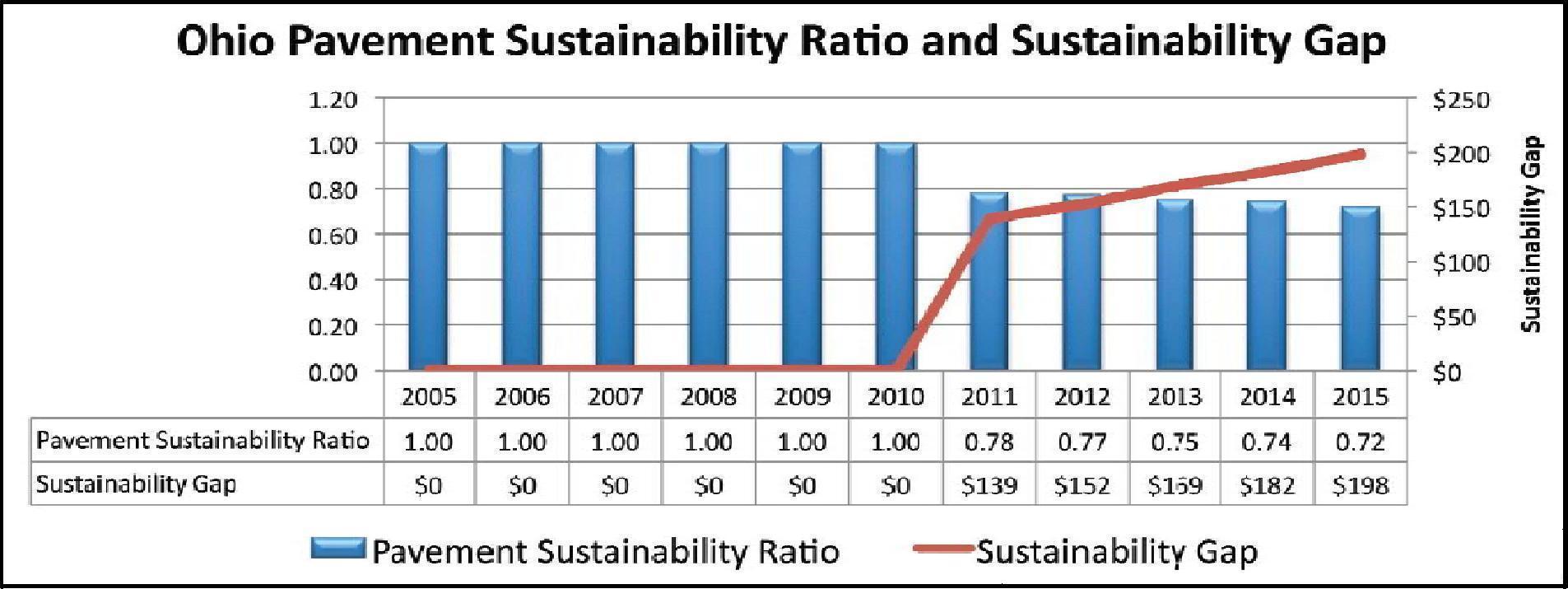
The financial information and the pavement condition forecasts provided in 2006 allow the illustration of a Pavement Sustainability Ratio for Ohio for this period of 2005-2015 as seen in Figure 19. It is a calculation of the amount budgeted, divided by the amount needed which results in the following as shown in Figure 19. It illustrates that from 2005 to 2010, the level of investment is adequate to sustain pavement conditions at ODOT?s targets. With expenditures relatively flat and materials costs forecast to rise, the Pavement Sustainability Index falls from 1.0 - adequate - to .78, or 22 percent below the amount necessary to provide stable, sustainable pavement conditions. Commensurately, a "Sustainability Gap" is illustrated on the secondary vertical axis and represents a cumulative gap of $838 million over the forecast period.
The Ohio DOT produces a long-term pavement condition forecast that is updated monthly and updated its Business Plan for the 2008-2009 and 2010-2011 biennium to address the earlier forecasts of impending pavement shortfalls. Table 13 depicts the total pavement expenditures for 2010 forecasted through 2017 as updated in the 2010-2011 Business Plan. They illustrate that ODOT increased pavement expenditures substantially, by an average of $109 million annually from 2010-2017, with a commensurate closing of the Sustainability Gap and the achievement of its pavement targets.
| Ohio Pavement Expenditure (Actual and Forecast) 2010-2012 Business Plan | ||||||||||
|---|---|---|---|---|---|---|---|---|---|---|
| Pavement Preservation Program | 2008 | 2009 | 2010 | 2011 | 2012 | 2013 | 2014 | 2015 | 2016 | 2017 |
| Pavement Preservation Budget | $581 | $578 | $484 | $612 | $676 | $674 | $709 | $742 | $776 | $812 |
| Priority System Acceptable | 98% | 98% | 98% | 98% | 97% | 98% | 98% | 97% | 97% | 96% |
| General System Acceptable | 95% | 96% | 96% | 96% | 96% | 95% | 95% | 94% | 92% | 88% |
| Urban System Acceptable | 97% | 98% | 98% | 98% | 97% | 97% | 97% | 96% | 94% | 91% |
| (expenditures in $millions) | ||||||||||
Table 14 illustrates the amended spending plan for 2010 through 2017 which was adopted in 2010 to address the under investment in pavements. As seen in Table 14, spending rose by between $139 million in 2011 to as much as $296 million in 2017 to fill the "sustainability gap" and to achieve the target of a Pavement Sustainability Ratio of 1.0. The calculation of the PSR and the computation of the delta to close the gap illustrate clearly the degree of additional investment necessary to sustain the pavement assets at the targeted condition through 2017. In 2006, ODOT forecasted the gap that was likely to occur if inflation continued as predicted. In 2010, when the effects of inflation had not diminished, ODOT increased pavement spending. If ODOT had been unable to re-direct the resources into the pavement program, the PSR would have reported to policy makers the future consequences of the under-investment and the relative size of the underinvestment.
| 2005 | 2006 | 2007 | 2008 | 2009 | 2010 | 2011 | 2012 | 2013 | 2014 | 2015 | 2016 | 2017 | |
|---|---|---|---|---|---|---|---|---|---|---|---|---|---|
| PSR Based on 2006 Pavement Budget | 1.00 | 1.00 | 1.00 | 1.00 | 1.00 | 1.00 | 0.78 | 0.77 | 0.75 | 0.74 | 0.72 | ||
| PSR Based on 2010 Budget | 1 | 1 | 1 | 0.91 | 0.96 | 1.18 | 1.04 | 0.97 | 1.00 | 0.98 | 0.96 | 1 | 1 |
| Expenditure Delta | $0 | $0 | $0 | $0 | $0 | $0 | $139 | $152 | $167 | $182 | $198 | $260 | $296 |
| (in $millions) | |||||||||||||
ODOT balanced several ever-changing variables to develop the updated 2008-2017 budget estimate and pavement forecast. It noted that inflation continued to be a concern but that it had subsided substantially, which reduced the impacts of material costs that were experienced in the earlier Business Plan. However, rising costs on top of the already significant price increases of the past years remain a substantial influence on the pavement program. ODOT further reduced its Major New Construction Program, or the capacity-adding projects, in order to address the pavement gap.
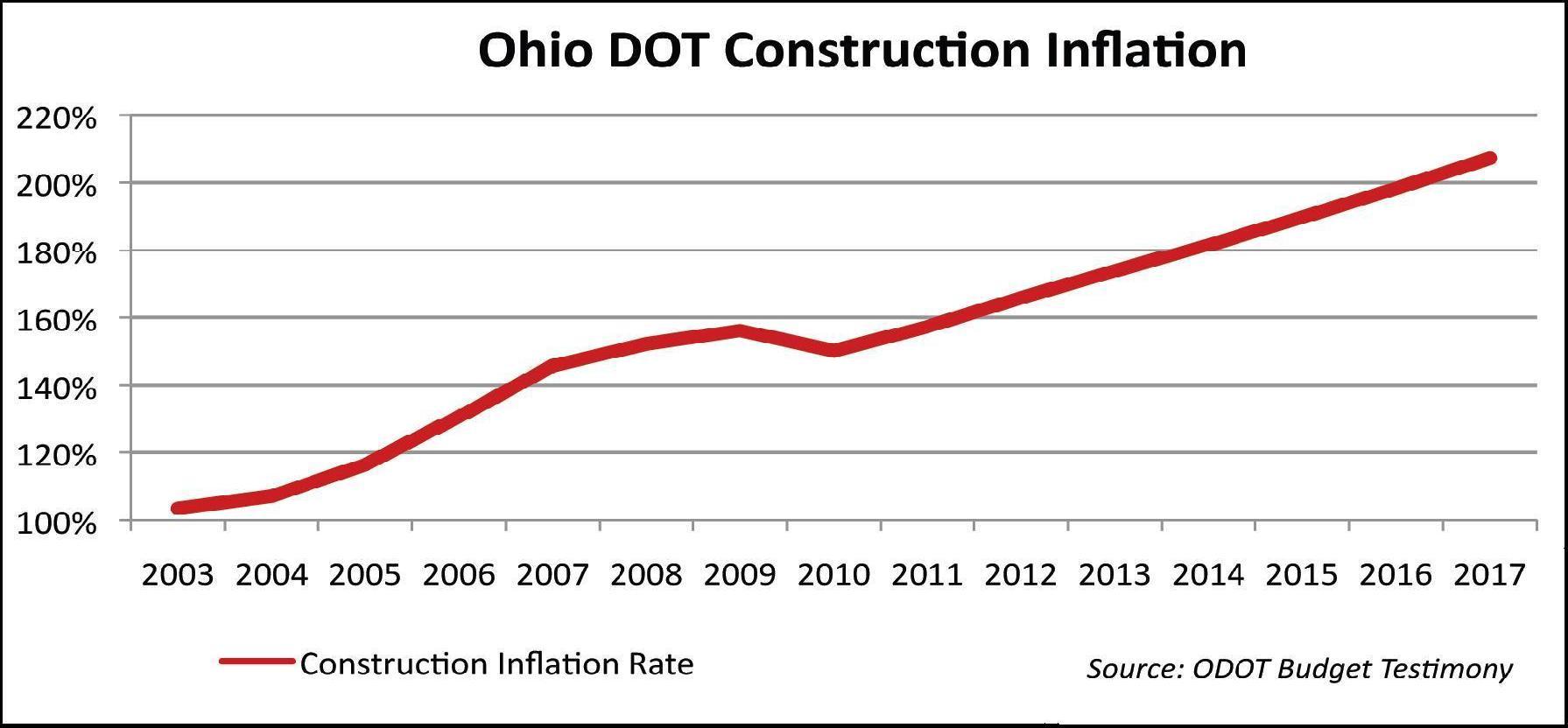
Figure 20. Construction inflation influenced investment needs.
A positive mitigating factor has been the increased service life Ohio has gotten from its pavements. Rates of annual degradation of untreated pavements have improved from a statewide average of 3.3 PCR points annually in the 1990s to as low as 2.5 percent PCR declines in the early 2000s. The difference equates to a 24 percent improvement in the longevity of the average pavement. In an annual pavement report, ODOT attributes improved pavement performance to a number of strategies, including tightened specifications, expanded preventive maintenance and enhanced decision making on treatment selection.
The granularity of the Ohio analysis allows for drilling into the underlying conditions that influence overall statewide pavement performance. This ability to "drill down" would allow the creation of a Pavement Sustainability Ratio for each district, each county or for any other subdivision, such as the highways within a Metropolitan Planning Organization (MPO) boundary. This granularity would allow an ODOT District or the neighboring MPOs to report on the PSR and total Asset Sustainability Index of its region. With the magnitude of a PSR known, the State, district or MPO could adopt long-range programming and pavement preservation strategies to sustain the pavement inventory.
In another example, the report generates a Pavement Sustainability Ratio using data from the Utah Department of Transportation (UDOT).
UDOT is considered to be one of the agencies with leading asset management processes and practices. As such, it provides the type of sophisticated long-term asset management forecast necessary to generate a credible Pavement Sustainability Ratio. The agency has a mature asset management approach that includes systematic and cost-effective maintenance, preservation, rehabilitation and operation of its physical assets. The UDOT Transportation Asset Management (TAM) approach tries to efficiently balance budget constraints, national issues, environmental priorities and public expectations in aligning its practices and applying asset management principles. With approximately 6,775 center lane miles (CLM) of roadway network to manage, the agency has successfully combined engineering, economics and sound financial planning with sound business practices in its decision-making.
To efficiently prioritize and manage its network the DOT has categorized the road network into four tiers based on the Annual Average Daily Traffic (AADT).
The four tiers/categories are:
These four tiers are sometimes combined for analysis purposes into three related categories, the Interstate, NHS and Non-NHS.
UDOT uses several factors (Condition Indices) to track the overall condition and performance of the roads. The Overall Condition Index (OCI) is the average of four primary Condition Indices. For asphalt, these are Ride, Rut, Environmental Cracking and Wheel Path Cracking. For concrete, these are Ride, Joint Faulting, Joint Spalling and Slab Cracking.
The agency has a strategy of "Good Roads Cost Less" (GRCL). Some of the interstate and level 1 road sections/segments have deteriorated to a state where they need minor and major rehabilitation. These roads will be managed on a "worst first" basis and are kept in serviceable condition through "Band-Aid" treatments until they can be reconstructed. However, the agency focuses on preservation of the roads that are in good condition to ensure that they continue to be in good condition. The preservation focus is to take care of the system to ensure sustaining its condition as "good" for the long-term.
UDOT has a strategic approach to financial planning as well as to engineering and implementation to address the long-term performance and sustainability of transportation assets. The strategy includes designing perpetual pavements on new capacity and pavement reconstruction projects. The agency defines perpetual pavement as "a pavement designed for a 50 year structural life, which will require a program of surface seals at set intervals throughout that 50 year life of the pavement. A perpetual pavement should not require any major rehabilitation or reconstruction work for the life of the pavement."
UDOT?s preservation treatment includes corrective maintenance, routine maintenance, preventive maintenance and minor rehabilitation. Corrective maintenance addresses immediate concerns of safety or pavement integrity and restores the pavement from unforeseen conditions to serviceable levels. Routine maintenance involves pro-active day-to-day activity to maintain and preserve pavement conditions at satisfactory levels. Preventive maintenance involves improving functional pavement conditions and extending the service life of the pavement. These are normally done on the surfaces of structurally sound pavements in good to fair condition and are lower-cost time-based treatments. The DOT's rehabilitation improves the pavement structure and addresses structural enhancements that extend service life or improve load-carrying capacity. Minor rehabilitation mainly addresses functional restoration of pavement surfaces due to age-related environmental cracking. Major rehabilitation usually increases pavement thickness to increase strength, addresses structural enhancements and accommodates increased traffic loading. Reconstruction replaces the entire existing pavement structure with similar or increased pavement thickness, thereby addressing pavements that have failed, become obsolete or have sub-grade issues.
In general, UDOT has put in place practices that help long-term sustainability of its transportation assets. These practices involve doing a Structural Overlay and Surface Seal in the 15th and 30th year. In between these two, alternate treatments of Surface Seal and Surface Rejuvenation are done every 3 years to sustain the condition of the pavement for 50 years.
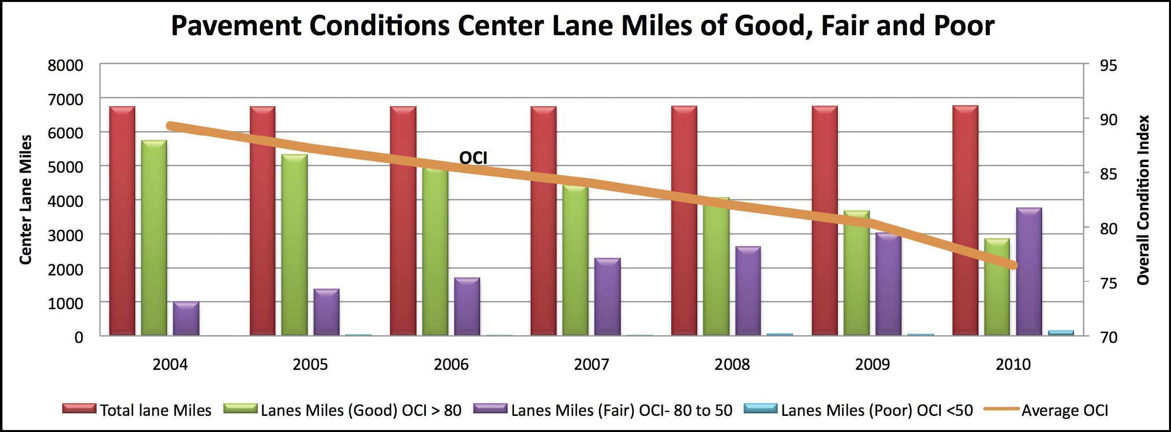
The historic trend of UDOT?s pavement conditions are as shown in Figure 21. Figure 21 shows that the Overall Condition Index of the network is falling from 89.3 in 2004 to 76.5 in 2010. The number of center lane miles in "poor" condition is increasing from 3.73 in 2004 to 146.97 in 2010.
Figure 21: Utah pavement conditions over time.
Agencies are currently challenged with making the right decisions on where to invest and how much to invest in their transportation assets. With limited funds, priorities will have to established and trade-offs will have to be made, both across asset categories as well as within asset categories. Under such circumstances, some assets will suffer from under-investment. The goal is to ensure long-term sustainable management and maintenance of the transportation assets and therefore, to ensure that any under-investment occurs in areas of least impact. Under investment, if applied selectively, may result in poorer condition and performance of some of the assets or if applied across the board, can result in poorer conditions even for high-priority assets. The computation of a Pavement Sustainability Ratio quantifies and brings to the forefront the projected results based on anticipated investment levels. It facilitates and triggers objective trade-off decisions and helps in better financial planning with the goal of making optimal use of available funds.
Figure 22: Utah pavement budget versus condition.
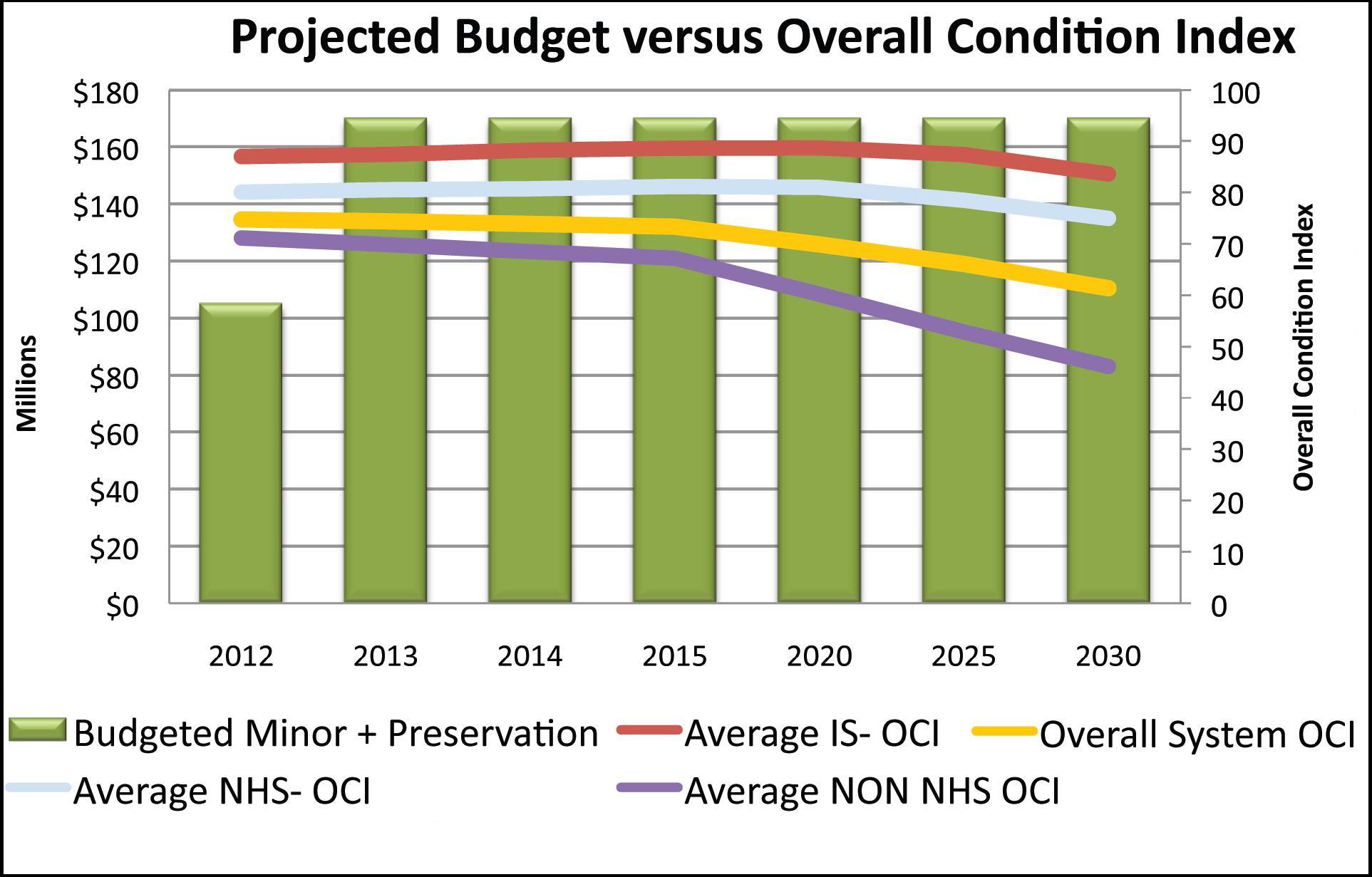
The discussion below focuses on the condition of the roadway network as well as budgets available and required to manage and maintain optimal pavement conditions. The information is used to compute a Utah PSR.
Figure 22 shows the Overall System Condition (OCI) of the different tiers of the roadway network based on projected funding for years from 2012 to 2030.
The figure shows the Overall System Condition (OCI) index falling from 74.72 in 2012 to 61.4 in 2030. Figure 22 also shows the OCI for the different tiers of roads in Utah. In the trade-off required by the budget constraints, the different priorities assigned to the three tiers (Interstate, NHS and Non-NHS) of the system are reflected in the difference in the condition of these tiers for the analysis period.
The condition for the Interstate system drops from an OCI of 87.0 in 2012 to an OCI of 83.6 in 2030, the condition for the NHS drops from an OCI of 80.04 in 2012 to an OCI of 74.94 in 2030 and the condition index for the non-NHS drops from an OCI of 71.13 in 2012 to an OCI of 46.16 in 2030.
Figure 22 also shows how the agency is using the available budgets and making trade-offs in managing and maintaining the performance and condition of the roadway network. The approach used gives higher priority to the more heavily used roads and to those carrying heavier loads as compared to those that have lesser traffic and carry lighter loads.
The highest priority is being given to the Interstate system. Second priority is given to the NHS system that is more used than the non-NHS. The third priority is given to non-NHS, the lesser used of the three systems.
Another way to depict the long-term consequences or outcomes of investment decisions is to measure backlogs of needed treatment.
Backlog is the term being used in this document for the roadway sections that require treatment but do not receive maintenance or rehabilitation activity.
Figure 23 shows the backlog of Interstate, NHS and non-NHS systems for the period starting in 2012 through 2030. When there are fewer constraints with availability of funds by moving funds across the different fund categories, agencies can be more liberal in performing preservation and maintenance activities on all tiers of pavements. As funds become more limited, ensuring sustainable performance-based management of assets requires prioritizing and making trade-offs between how much to spend and when to spend monies on the Interstate, NHS and non-NHS system.
Figure 23: Backlog of pavement treatments.
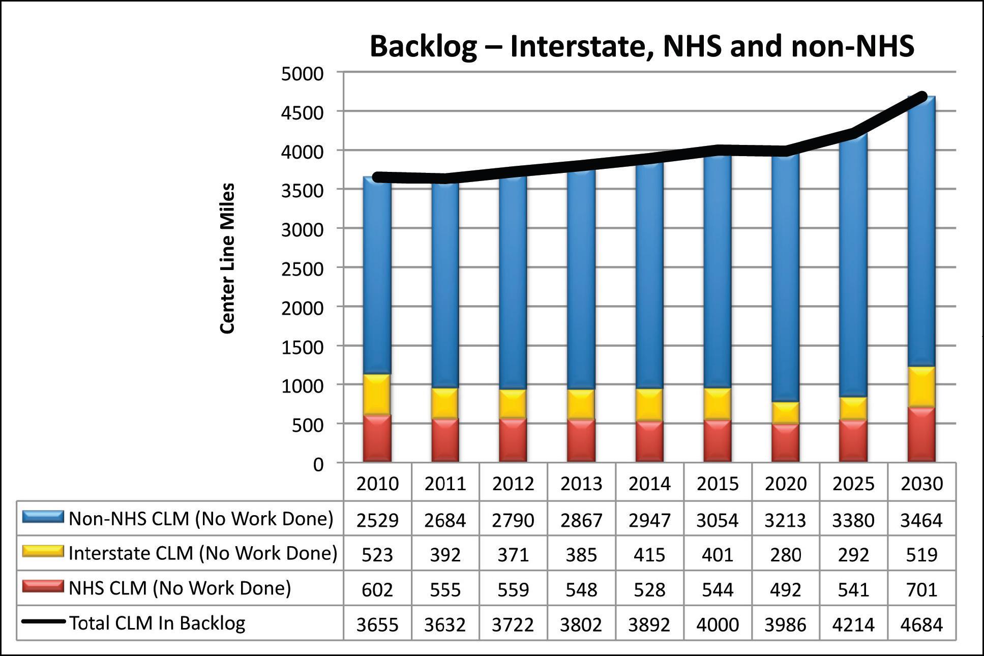
Figure 23 shows that the backlog on the Interstate system is being kept to a minimum, the backlog on the NHS is higher and the backlog of miles not addressed by maintenance and rehabilitation activity in the non-NHS system increases from 2,530 CLM in 2012 to 3,456 CLM in 2030. Figure 23 also shows that the total backlog increases from 3,655 CLM in 2012 to 4,685 CLM in 2030.
Figure 24 shows the condition of the interstate system after trade-offs have been applied to optimize the use of available funds. It shows that the Interstate in "good" condition increases from 1,481 CLM in year 2011 to 1,503 CLM in 2012. The overall CLM for interstate in "good" condition varies minimally between 1,490 CLM and 1,450 from 2013 through 2015. The CLM in "good" condition increases from 2020 through 2025. In 2030 the CLM in "good" condition decreases while the CLM in "poor" condition increases.
Figure 24: Utah Interstate pavement condition trends.
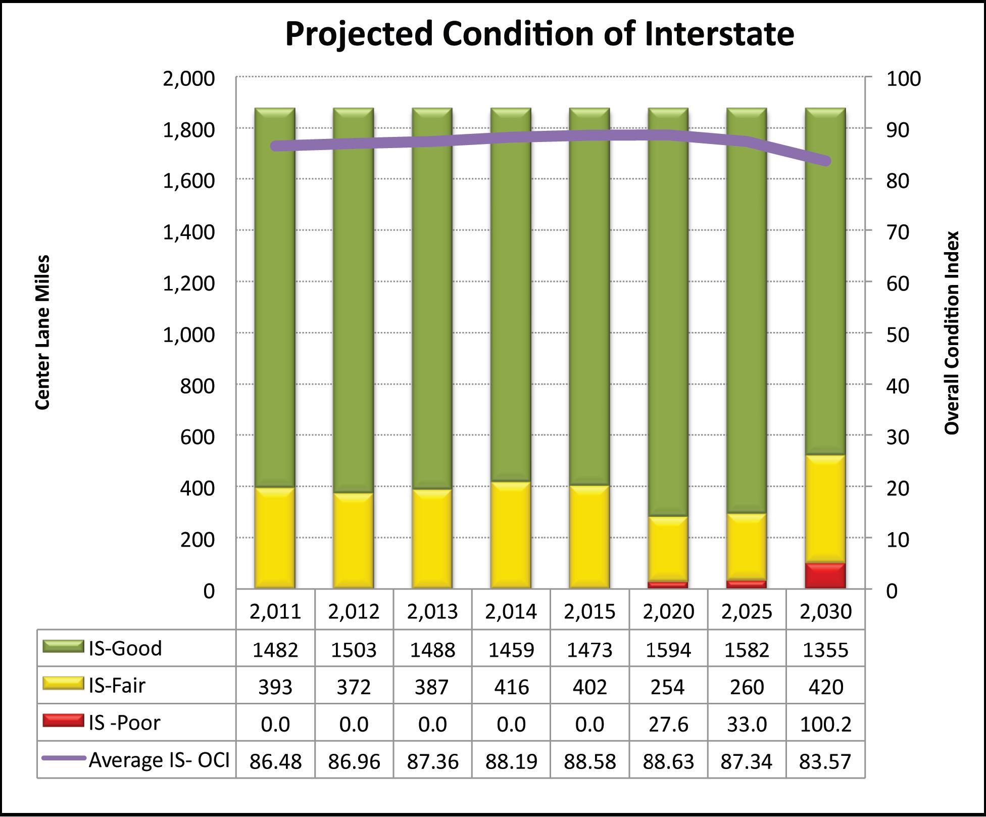
Figure 24 also shows the corresponding change in the average OCI for the interstate system from year 2011 to 2030. It shows the OCI for the interstate system improving from 86.48 in year 2011 to 88.63 in year 2020.Figure 24 also shows that the projected OCI drops to 83.57 in 2030.
Figure 25 shows the number of CLM for the NHS from 2011 to 2030 in "good", "fair" and "poor" condition. It also shows the statewide average OCI improving from 79.47 in year 2011 to 80.04 in year 2012 and remaining around 80 from year 2012 through year 2020 and then dropping progressively to 74.94 by 2030.
Figure 25: NHS conditions and trends.
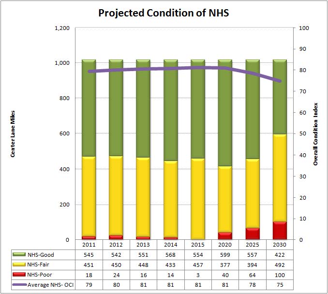
Figure 26 shows the condition of the non-NHS in "good", "fair" and "poor" from 2011 through 2030. It shows the CLM in "fair" condition decreasing from 2635 in year 2011 to 1103 in year 2030. It shows a corresponding increase in the "poor" condition for the same period with CLM of "poor" condition increasing from 155.2 to 2526.9. The figure also shows the number of CLM in "good" condition decreasing from 1059 in year 2011 to 219 in year 2030. This overall fall in system condition is reflected in the OCI decreasing from 72.3 in 2011 to an OCI of 46.165.
Figure 26: Non-NHS condition and trends.
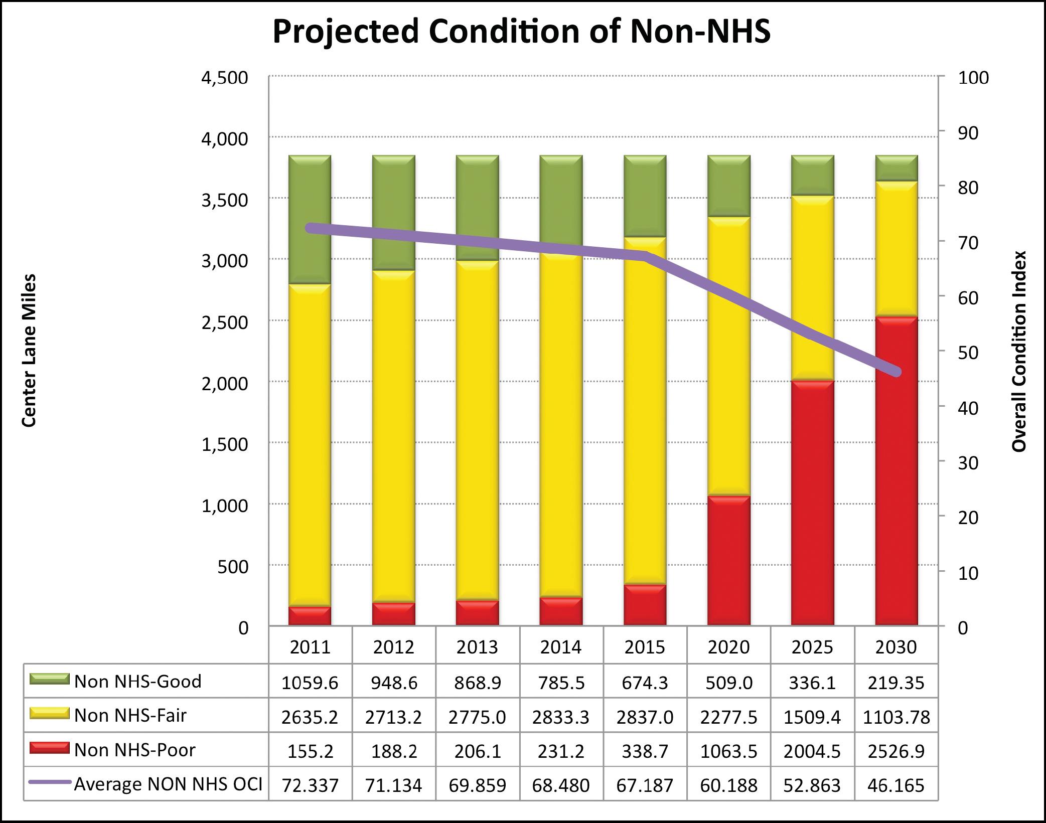
Figure 27 shows the optimal long-term conditions that can be achieved for the Interstate System (IS), NHS and non-NHS systems and the budget required to sustain the optimal OCI for the system from 2011 through 2030, assuming that there are no budget constraints.
Figure 27: Budget need for optimal conditions.
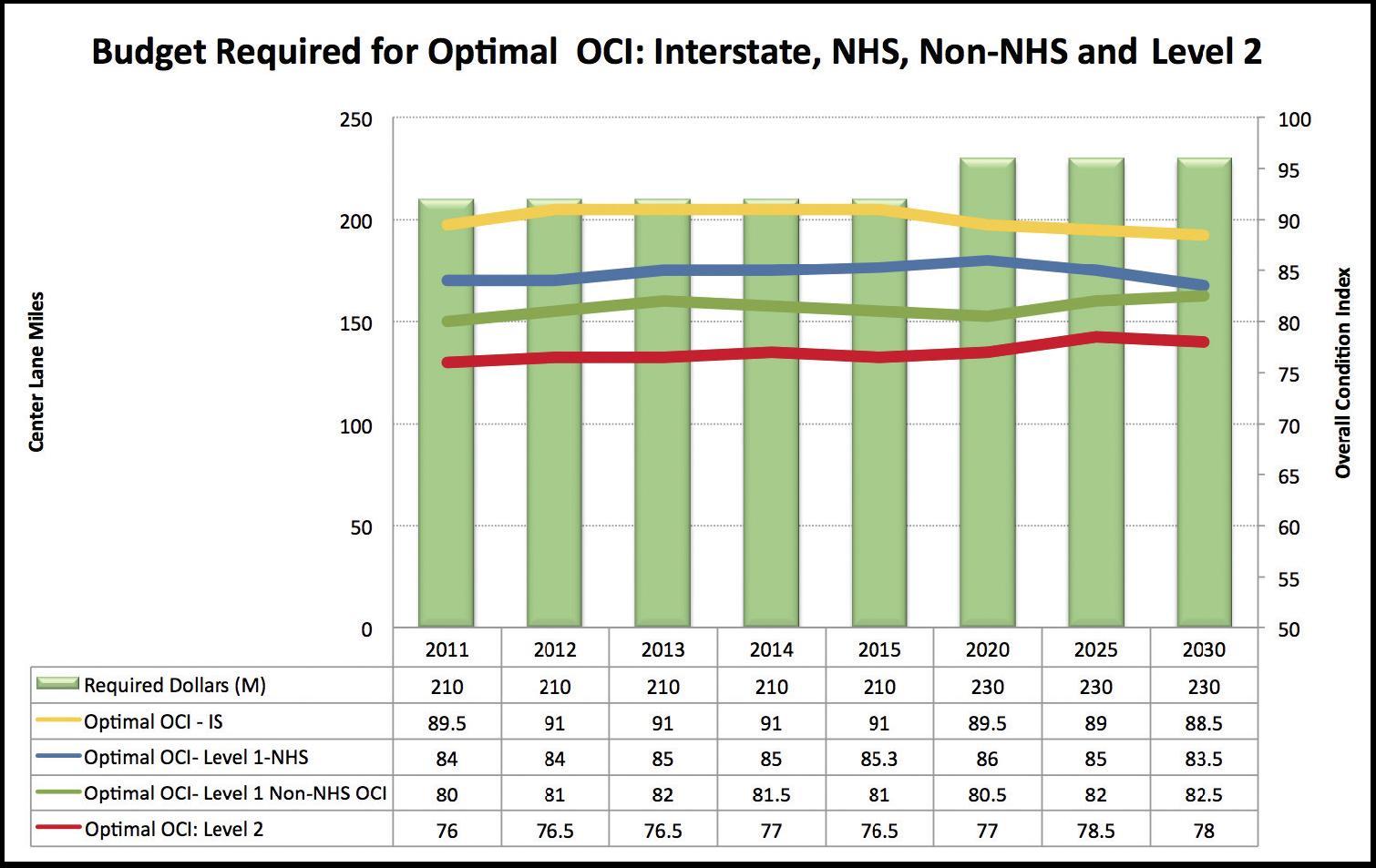
Figure 27 shows how with appropriate long-term financial planning an agency can compute the optimal amount of funds required to sustain the long-term performance and condition of the roadway network.
To identify the optimal conditions that can be achieved for a long-term period of nearly 20 years in the future, different scenarios of conditions that can be achieved for different budget amounts for each tier of the roadway are generated. These multiple scenarios are then analyzed to identify the minimum budget amount required to achieve and sustain optimal pavement conditions in the future.
Figure 27 shows the optimal condition that can be achieved for each of the tiers of the roadway. The total annual amount required to sustain the optimal OCI is approximately $210 million in years 2110 through 2015. The budget required to sustain the optimal OCI beyond year 2015 increases to $230 million dollars annually.
Figure 28: Utah pavement sustainability ratio.
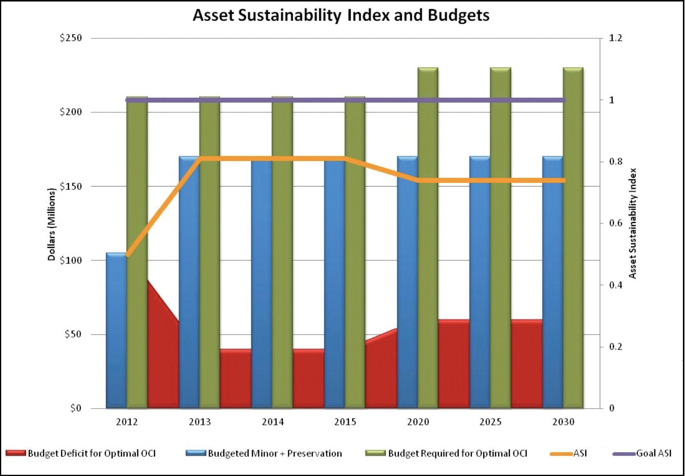
The available and required budgets (for optimum OCI) as discussed above are consolidated in Figure 28 along with the budget deficit to maintain optimum conditions. Figure 28 also depicts the Goal PSR (assuming optimum budget availability) as well as the projected PSR based on available budgets.
A Pavement Sustainability Ratio is a metric calculated by dividing the amount budgeted for pavement maintenance and preservation over time by the amount needed to achieve a specific pavement condition target.
This PSR= 1 is shown in purple in Figure 28. The PSR is computed as:
| Pavement Budget Pavement Needs |
= Pavement Sustainability Ratio |
Figure 28 shows the currently projected PSR based on available budgets in orange. The PSR is 0.4 in 2012, showing a 60 percent shortfall from optimum needs. It increases to 0.8 in 2013 and remains at 0.8 until 2015. After 2015, the PSR drops from 0.8 to 0.74 in 2020 and remains at 0.74 through year 2030.
As shown in the UDOT example, a Pavement Sustainability Ratio can be computed using the asset condition forecasts and related investment needs generated from a mature U.S. State asset management process. The example also illustrates that the PSR thus is a tool that can be effectively used to consolidate the analysis of the overall system conditions, required budgets to maintain optimum system conditions, and available budgets (representing fiscal constraints) into a single metric. The PSR can therefore also be used to effectively illustrate and communicate to all stakeholders the budget status and investment needs required to maintain optimum system conditions.
This example illustrates how a Pavement Sustainability Ratio could be calculated using a third State's data. This analysis also illustrates how long-term system forecasts can be used to illustrate the consequences of tradeoffs.
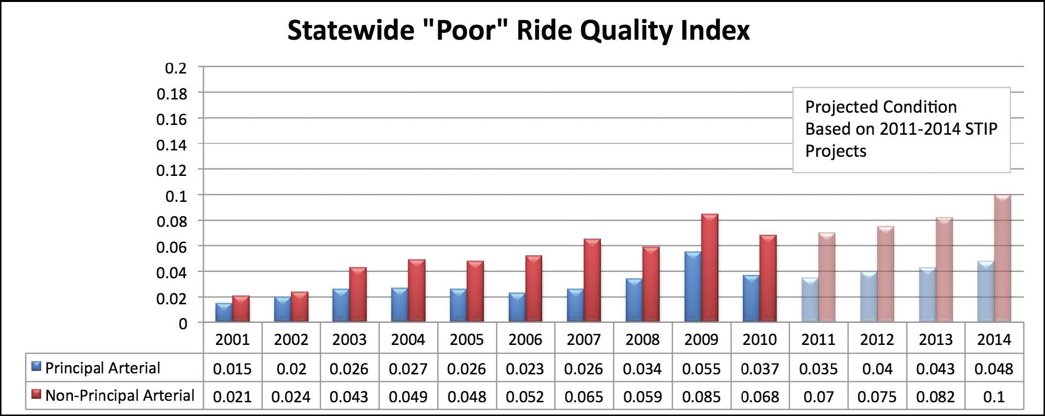
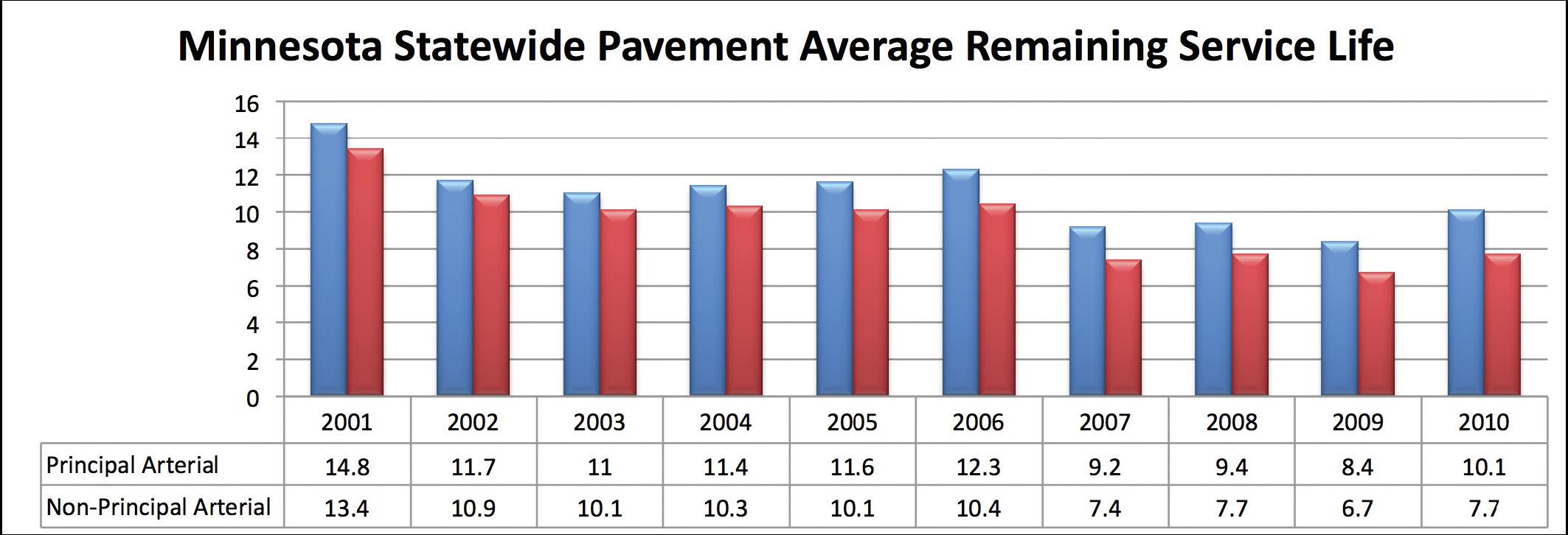
Figures 29, 30 and 31 below from the Minnesota DOT (MnDOT) are typical of the type of information that often is portrayed by States and which could contribute directly to a Pavement Sustainability Ratio. Figure 29 illustrates that the agency has struggled since 2001 to reach its pavement-condition targets and that it has had to accept gradually lowering conditions, particularly on its Non-Principal Arterials. Figure 30 illustrates that the percentage of "Poor" Ride Quality Index miles also has steadily increased and are forecast to rise significantly in the next four years. Even more germane to the concept of an Asset Sustainability Index is Figure 31. It illustrates that the Remaining Service Life of the State's pavements has steadily declined, by as much as 43 percent between 2001 and 2010 for the Non-Principal Arterials. Figures 30 and 31 illustrate the type of long-term implications that GASB 34 and TAM guidelines seek to capture. Those figures show the erosion in the "robustness" of the pavement inventory. With its significantly reduced Remaining Service Life, the pavements have less "elasticity" to sustain a temporary budget reduction, to withstand increased traffic loadings or other impacts. In addition, future costs likely will rise as it is more expensive to rehabilitate a deteriorated pavement than to maintain a good one. As such, the "value" of the 2014 pavement inventory is significantly less than the value of the 2001 inventory that had a greater Remaining Service Life. In simple terms, it would be analogous to the value of a car with 50,000 miles compared to one with 71,500 miles, or 43 percent more miles.
Figure 29: MnDOT "good" ride quality.
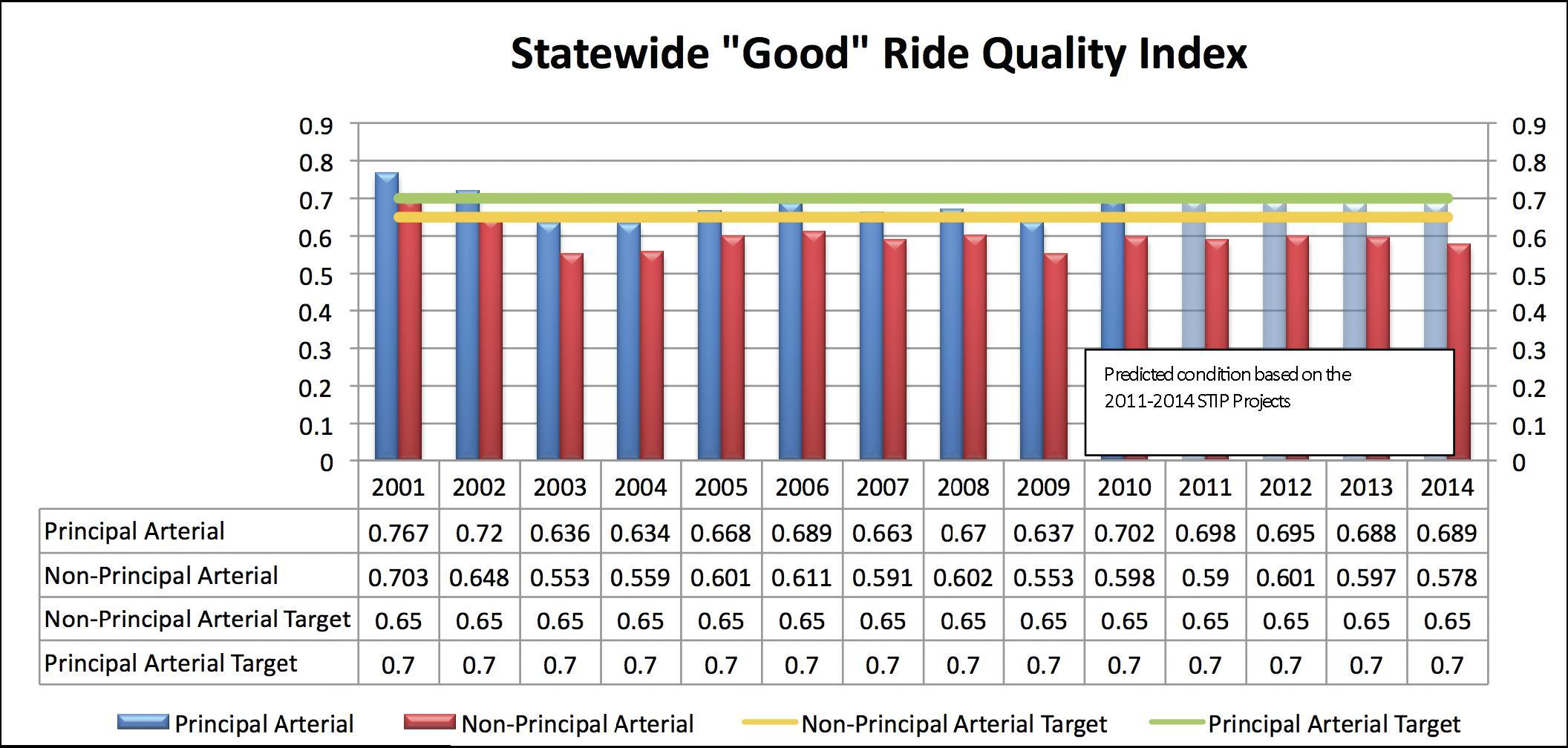
Figure 30: MnDOT "poor" ride quality index.
Minnesota defines Remaining Service Life as the number or remaining years until a pavement declines to a 2.5 out of 5 in its Ride Quality Index. The rating of 2.5 indicates the pavement is in need of rehabilitation to provide an acceptable ride. The terminal condition of 2.5 does not indicate the road is unusable, only that its condition cannot be restored without significant rehabilitation.
Figure 31: MnDOT remaining service life.
Minnesota's data and its analyses clearly inform policy makers of the pavement-deterioration trends and their causes. The first important trend is declining overall revenue forecasts.
Figure 32: MnDOT declining program projections.

As Figure 32 illustrates, capital revenue forecasts decline substantially as fuel tax receipts stagnate, operating costs rise, less bond income can be afforded and Federal apportionments remain unclear.
Figure 33: MnDOT's declining pavement investment levels.
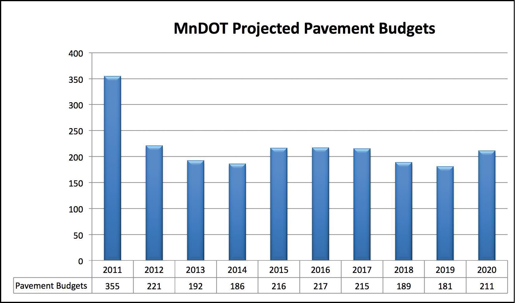
Figure 33 illustrates that commensurate with the overall decline in spending, pavement expenditures will fall. This decrease in pavement spending comes at a time of enhanced investment in bridges, following the collapse of the I-35 Bridge in Minneapolis. A special legislative directive requires the department to replace 120 fracture critical or structurally deficient bridges. Approximately 32 percent of all STIP funding from 2011 to 2020 will be devoted to bridges, with two-thirds of that devoted to these structures.[7] The results are predicted to be that the percentage of bridges meeting their structural condition goals will rise from 87 percent in 2009 to 89 percent in 2014, with conditions through 2020 projected to remain above the target of 84 percent.
MnDOT predicts that it will meet several important long-term targets in the 2011-2020 planning period. Targets it expects to meet include:
However, the expected lower revenue and investment-tradeoff decisions will result in the department being unable to meet its pavement targets particularly on the Non-Principal Arterials. The number of State highway miles with good pavement conditions will decrease and the number of State highway miles with poor pavement condition will increase from 990 miles in 2009 to 2,528 by 2019.
The estimated cost of the needed investment to sustain the Minnesota pavement conditions was not directly available for this report. MnDOT's process for generating pavement needs was between annual planning cycles and the necessary analyses to estimate the financial need for pavements to sustain conditions was not available. However, the Minnesota data that were available illustrate that with some additional computer runs, that MnDOT could produce a pavement sustainability ratio as described in this report. The type of analysis possible with the MnDOT processes likely would illustrate that while bridge conditions were sustainable, the pavement conditions are not at current investment levels. Substantial pavement investment increases will be necessary, and a Pavement Sustainability Ratio would illustrate the magnitude and cost of the needed investment.
[6] Ohio Department of Transportation, "Asset Management Peer Exchange," document, Sept. 7, 2004, at a TRB workshop.
[7] Minnesota DOT, "Highway Investment Plan Annual Update 2011-2011" Table 1, pg. ii.
| << Previous | Contents | Next >> |