| << Previous | Contents | Next >> |
State transportation officials have long experience in measuring infrastructure condition. They produce extensive inventories of bridges, pavements, and roadside assets and they have tracked their condition over time. In cases where mature management systems are in place, the highway officials often create forecasts and scenarios to evaluate different investment options.
The Asset Sustainability Index concept allows transportation officials to portray their infrastructure condition information in additional ways to communicate more effectively about the consequences of current trends. By its very nature, highway infrastructure is a long-term asset whose future condition is dependent upon long-term actions. A long-term perspective is even more important when an entire network or system of assets is being evaluated.
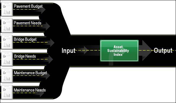
In concept, the Asset Sustainability Index should be simple to grasp. As seen in Figure 1, it is a calculation of the need divided by budget for various highway infrastructure categories. For the purposes of this report, it will be defined as:
An Asset Sustainability Index is a composite metric computed by dividing the amount budgeted on infrastructure maintenance and preservation over time by the amount needed to achieve a specific infrastructure condition target.
Stated mathematically, it is:
| Amount Budgeted Amount Needed |
= Asset Sustainability Index |
In the definition, the terms "maintenance" and "preservation" are used generically to include all preventive, reactive, rehabilitative and even replacement activities that contribute to the achievement of an infrastructure condition target. The terms "maintenance" and "preservation" are not intended to be synonymous with any terms relating to eligibility of Federal Highway Administration or other funds. The index also relies on "budgeted" not "spent" or "obligated" funds. The index is a planning and long-term programming metric. As such it assumes a high correlation exists between the amount budgeted for a program and the amount actually spent over time. Although the amount budgeted for a program and the amount spent for it may vary year to year, over time a strong correlation is assumed for the ASI. A separate discussion regarding inordinately costly items, such as rehabilitation of major bridges or pavements, is addressed later. Also addressed later in this chapter is a discussion of how to capture "need" in a credible and replicable way.
Figure 3: Inputs to the Asset Sustainability Index.
An ASI of 1.0 is considered optimum because expenditures match need. Economically, a perfect match of need and expenditure is most efficient because it preserves infrastructure for the lowest cost over time and excess spending above 1.0 can be redirected to other needs. The budgeted amount is the numerator and the need the denominator to allow the representation of 1.0 to be optimum. Any fractional number below 1.0 illustrates a deficit in investment and a number above 1.0 illustrates excess spending. "Excess" however, may be needed temporarily to eliminate backlogs in deficiencies. Again, as the ASI is intended to be a long-term, planning metric the optimum amount of investment is that which is needed to sustain conditions at a targeted level over the long-term. At the end of this section is a discussion of how "need" can be determined.
Webster?s Third New International Dictionary defines an index as, "a ratio or other number derived from a series of observations and used as an indicator or measure." The ASI is proposed to be used in a time series to measure trends. The time series is deemed to be important because of the long-term nature of infrastructure management and performance.
As an index, the ASI is proposed to summarize or comprise three ratios, a Pavement Sustainability Ratio, a Bridge Sustainability Ratio and a Maintenance Sustainability Ratio. They will have nearly identical definitions which are:
A Pavement Sustainability Ratio is a metric calculated by dividing the amount budgeted for pavement maintenance and preservation over time by the amount needed to achieve a specific pavement condition target.
| Pavement Budget Pavement Needs |
= Pavement Sustainability Ratio |
A Bridge Sustainability Ratio is a metric calculated by dividing the amount budgeted for bridge maintenance and preservation over time by the amount needed to achieve a specific bridge condition target.
| Bridge Budget Bridge Needs |
= Bridge Sustainability Ratio |
A Maintenance Sustainability Ratio is a metric calculated by dividing the amount budgeted for roadway maintenance needs over time by the amount needed to achieve a specific roadway maintenance appurtenance condition target. The ratio addresses capital expenditures, and can include labor and equipment costs depending upon the user?s practices.
| Maintenance Capital Budget Maintenance Capital Need |
= Maintencance Sustainability Ratio |
The capital items included in a Maintenance Sustainability Ratio could vary depending upon the definitions used by the highway agency. At the simplest level, they would include capital expenditures for guardrail, pavement markings, and signs. Depending upon the accounting and program practices of a department, it could include traffic signals, culverts, drainage items or other items. In the North Carolina DOT case study the definition of maintenance is much broader and extends to bridge and pavement items as well. For simplicity in this report, generally the capital items of guardrail, pavement markings and signs are included although that varies depending upon the available State data used in the examples. If a department desired, the necessary expenditures for labor and equipment also could be included. For instance, if it calculated that a given amount of labor, equipment and capital was necessary to sustain guardrail at a given targeted level, those three expenditure inputs could be used in the numerator and denominator for a Guardrail Sustainability Ratio. That ratio could be incorporated into the larger Maintenance Sustainability Ratio.
Generically, any of the three ratios could be called Asset Sustainability Ratios. The definition for an Asset Sustainability Ratio would be:
An Asset Sustainability Ratio is any asset-class-specific ratio of budget divided by the amount needed to sustain condition targets over the long-term and could refer generically to the Pavement Sustainability Ratio, the Bridge Sustainability Ratio or the Maintenance Sustainability Ratio.
A simple example of a Pavement Sustainability Ratio follows. A highway agency calculates from its pavement management process that a rational annualized program of preventive, reactive, rehabilitative and replacement projects necessary to sustain its rural highway system pavement conditions is $200 million annually. It divided the amount it budgets for rural system pavements by $200 million to calculate 1 year?s PSR for rural pavements. As seen in Table 1 the amount budgeted and the amount needed in 2000 both are $200 million, therefore, the PSR is 1.0.
| 2000 | 2001 | 2002 | 2003 | 2004 | Rate of Growth | |
|---|---|---|---|---|---|---|
| Budgeted | $200 | $206 | $212 | $219 | $225 | 3% |
| Needed | $200 | $208 | $216 | $225 | $234 | 4% |
| PSR | 1.0 | .99 | .98 | .97 | .96 |
The agency has balanced its expenditures and needs for rural pavements. As a result, for that year its rural pavements are sustainable. However, as the last column of Table 1 indicates, the highway agency increased rural pavement expenditures by 3 percent annually, but inflation created 4 percent annual growth rate in costs. Need by 2004 grew to $234 million but budgets were only $225 million. Commensurately, the PSR fell to .96
| 2000 | 2001 | 2002 | 2003 | 2004 | Annual Rate of Change | |
|---|---|---|---|---|---|---|
| Budgeted | $200 | $206 | $212 | $219 | $225 | 3% |
| Needed | $200 | $208 | $216 | $225 | $234 | 4% |
| PSR | 1.0 | .99 | .98 | .97 | .96 | 1.0% |
| Asset Valuation | $3,500 | $3,465 | $3,430 | $3,396 | $3,328 | 5% |
For budgeters, planners, programmers, legislators and similar parties interested in the long-term stability of the highway network, the PSR provides a relative, proportional indicator of the gap between need and investment for the pavement network. To add further relevance, additional metrics that are key inputs to or from the PSR can be included in the reporting process to provide additional insight. In 2000, the rural highway network was valued at $3.5 billion, gradually declining to $3.328 billion by 2004. In other words, this pattern of investment led to the State losing $172 million in "equity". The taxpayers owned $3.5 billion worth of rural highway assets in 2000 but the value of those assets declined to $3.328 billion in only five years as the pavements degraded and were not adequately repaired. The ability of the Pavement Sustainability Ratio and the Asset Valuation to illustrate the consequences of underinvestment increases with the time series.
Figure 4: Pavement Sustainability Ratio and valuation over time.
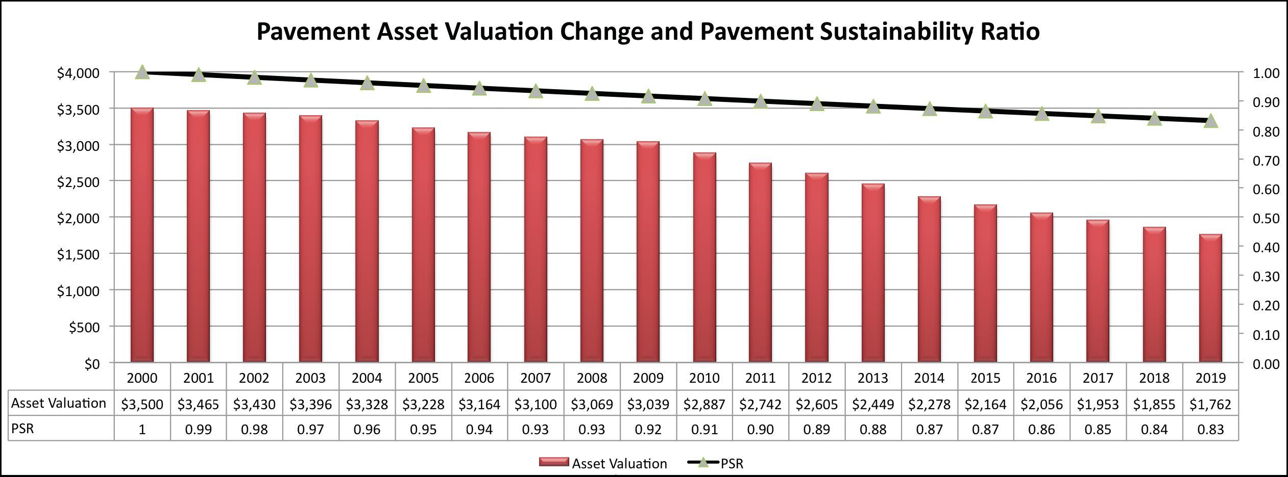
In Figure 4, the long-term consequences of what appears to be a relatively minor amount of under-investment each year become clearer. From 2000 through 2010 the PSR for rural highway system pavements only gradually declined from 1.0 to .91. Superficially, it appears that based on the PSR, that investment was only nine percent below optimum. However, over time that led to a steady decline in asset valuation. The rural highway system began with a value of $3.5 billion, declined to $2.887 billion by 2011 and is forecast to fall to $1.762 billion by 2019. Over the course of 20 years, the value of the highway agency?s rural pavement assets declined by 50 percent. This leaves future users with much less "equity", lower pavement conditions and a substantial backlog in investment required to restore the asset?s value and functionality.
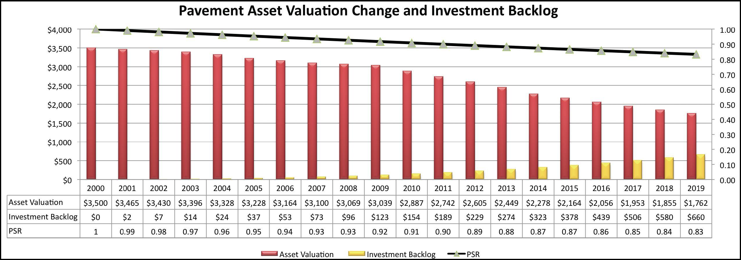
Figure 5: The "Sustainability Gap" or investment gap.
A ratio such as the PSR is intended to help budgeters "calibrate" a highway agency?s program. It allows budgeters to depict the amount of additional spending needed to achieve a specific condition target. Metrics such as average pavement condition, or miles of deficient pavements provide insight into the physical magnitude of pavement deficiencies. The PSR and its ASI help budgeters understand the financial magnitude of the "investment gap" or "investment surplus." As importantly, the sustainability metrics provide a simple way to communicate the adequacy of investment into a simple ratio. While concepts such as Remaining Service Life or Pavement Serviceability Index may be hard to communicate to a lay audience, the sustainability metrics are intended to provide simple ratios that indicate the degree to which investment is adequate or inadequate.
The fiscal component allows the PSR to support "triple bottom line" or "balanced scorecard" types of measurement systems. In the triple bottom line or balanced scorecard systems, multiple societal objectives are weighed. These can include environmental sustainability, infrastructure sustainability as well as financial sustainability. The PSR and ASI can feed into these types of mature performance measurement systems and can provide a financial order-of-magnitude perspective lacking from measures that only report upon infrastructure conditions, such as the Pavement Serviceability Index or International Roughness Index. The PSR or ASI is not proposed to replace those metrics, but rather to complement them.
By placing a monetary value on infrastructure through asset valuation, the under-investment in that infrastructure over time can be expressed as a loss of value to the society as a whole and as a "backlog" or "infrastructure deficit". As seen in Figure 5, the 20-year decline in PSR for this theoretical rural highway pavement inventory leads to a halving of the inventory?s value and a backlog of repairs of $660 million by 2020. Although theoretical, the inputs to this analysis are based upon inventory size, average treatment costs and asset values taken from later case studies referenced in this report. In this example, they are simplified for the purposes of illustrating the PSR and asset valuation concept.
The "backlog" or "infrastructure deficit" is an intentional focus of the sustainability metrics and asset valuation efforts. They are intended to focus attention upon the future or long-term consequences of underinvestment. They allow an organization to depict to policy makers whether current investment levels lead to sustainable infrastructure for future users. Just as greater expenditures than contributions create deficits in the Social Security or Medicare programs, continued underinvestment in infrastructure creates deficits that are not normally captured in traditional highway metrics. In the theoretical case study of Figure 5, a deficit of $660 million is accumulated. To address it, the highway agency must either accept lower condition standards or it must impose upon future users substantially higher costs.
The geometric progression of miles of deficiencies, the loss of asset value and the increase in backlog are attributable to the non-linear progression of pavement degradation once pavements deteriorate to a certain point.
Figure 6: Pavement deterioration curves.
Figure 6 (from the Federal Highway Administration?s Office of Asset Management, Pavements and Construction) illustrates the steep deterioration curve commonly seen in pavements once they reach a "poor" condition. Timely preventive and reactive treatments create substantial value by restoring pavements to a high condition and preventing the onset of the rapid deterioration commonly seen in poorly maintained pavements. As noted in Figure 6 and in other FHWA reports, timely preventive and reactive treatments can produce a very high benefit/cost ratio. Conversely, underinvestment leads to the missing of the optimal treatment-timing window for many pavements and leads to their concurrent rapid, non-linear degradation. It is the accelerating, non-linear degradation that underlies the analysis? rapid accumulation of deficient lane miles and the rapid growth in the cost of the backlog, or the accumulation of the "infrastructure deficit".
Another example of how an investment ratio can be calculated follows. This one is for guardrail, which is one component of the Maintenance Sustainability Ratio. Following this example, the "rolling up" of these individual ratios into an Asset Sustainability Index will be presented.
Figure 7: Guardrail sustainability ratio calculation.
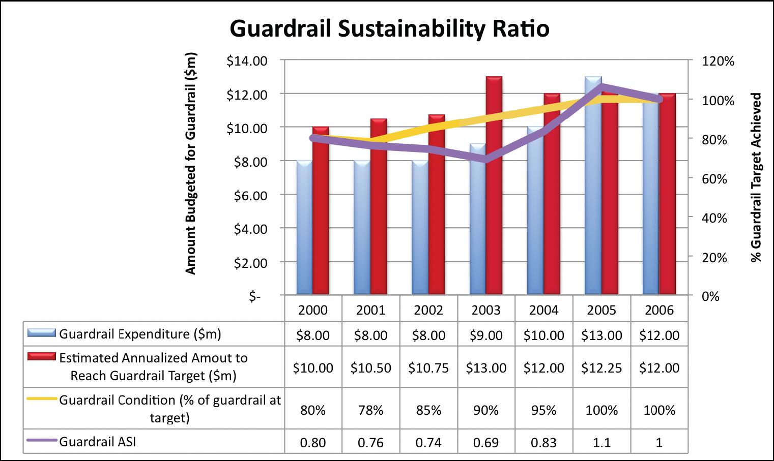
Figure 7 illustrates how a guardrail Sustainability Ratio would work. The blue bars and accompanying data table illustrate amounts budgeted for guardrail for a hypothetical highway agency. The red bars illustrate the needed level of investment to achieve the target. For instance in 2000, $10 million is needed but only $8 million is budgeted. The yellow trend line and table illustrate that the expenditures from 2001-2004 were below the needed amount to achieve the guardrail target. As a result, only 80 percent of the targeted condition level was met in 2000, falling to 78 percent in 2001. The corresponding Guardrail Sustainability Ratio is then .8 in 2000 falling to .76 in 2001.
| Guardrail Capital Budget Guardrail Capital Needs |
= Guardrail Sustainability Ratio |
Expenditures were increased beginning in 2003. As a result, the backlog was reduced and the amount invested in 2005 actually allowed the department to exceed its target. As a result in 2006 the department decreased expenditures to $12 million, matching the amount needed to achieve the goal. As a result, an ASI of 1.0, the desired level, was achieved.
Figure 8 illustrates that expanding the time series to include more years allows a long-term perspective on the necessary investment. Figure 8 illustrates that if budget year 2011 (highlighted in green and yellow) serve as the current year in which a guardrail budget is to be evaluated that the past expenditure and condition data illustrate the consequences of past investment decisions. Between 2000 and 2005, guardrail investment was inadequate, conditions declined and investment had to substantially increase to correct the backlog.
Figure 8: Long-term investment perspective.
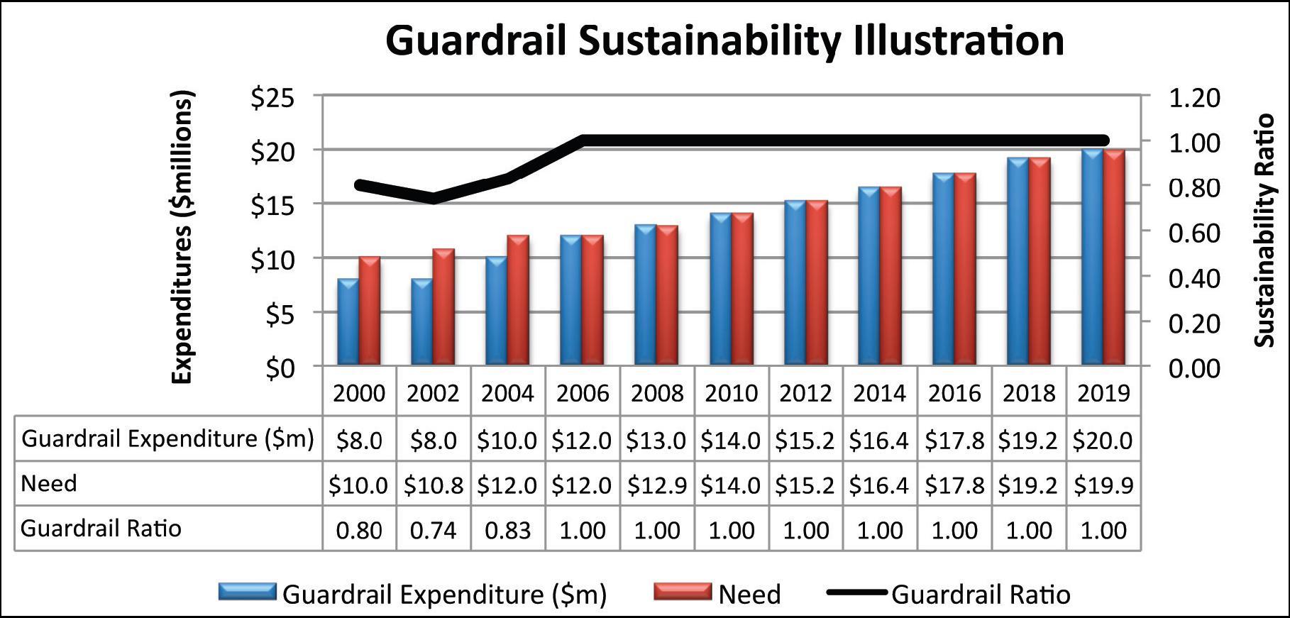
Budgeting forward, the agency assumes a 4 percent annual increase in guardrail costs and commensurately increases the forecast of guardrail expenditures from $14.60 million in 2011 growing to $19.98 million in 2019. This 20-year perspective provides insight for long-range plans, Statewide Transportation Improvement Programs and other longer-term budgeting and programming exercises. To achieve a 1.0 or optimum Guardrail Sustainability Ratio, the past history of under-investment is numerically and graphically illustrated. Commensurately, the investment needed to sustain conditions at the targeted condition level to the planning horizon year can be demonstrated.
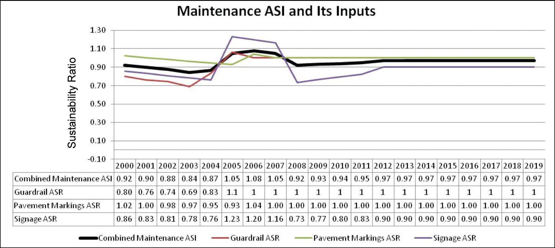
Creating a weighted index from various ratios becomes a simple arithmetic exercise. For the sake of this simple illustration, the Maintenance Sustainability Ratio is derived from the needs and budgets of guardrail, signage and pavement markings. As seen in Figure 9 the three areas of expenditure are summed, both for their need and for their budgets. Total budgets are divided by total need to illustrate how the Guardrail, Pavement Marking and Signage components comprise a Maintenance Sustainability Ratio.
Figure 9: Combining ratios into an index.
Similarly, the budget and needs of all pavement systems and bridge systems can be illustrated. With this type of reporting, not only can the sustainability of overall investment levels be evaluated but the granularity of reporting by infrastructure category allows the reporting to clearly indicate which infrastructure types are not meeting targets. As will be seen in the later case studies, in the current environment of greatly constrained budgets, States are making difficult tradeoffs. In at least two cases that will be illustrated, rural pavement conditions are deteriorating because limited highway agency funds are being invested to sustain conditions on the more heavily traveled major routes such as the National Highway System. In another State, bridge investment was substantially increased while pavement conditions declined.
The granularity of the ASI and ASRs as presented here allow for the reporting of the consequences by asset class of investment decisions. This granularity also is discussed in Chapter 8. There, the GASB 34 reports are discussed and how their lack of granularity by asset class can mask significant declines in important asset classes, such as pavements.
As noted, the sustainability ratio and indices are based on dividing the amount budgeted for infrastructure preservation by the amount needed. A strong emphasis is placed upon "preservation" as opposed to capacity. The intent of the ASI is to address condition, not performance.
A common process for determining the amount needed for infrastructure preservation does not exist in the United States. There is no standard template an agency can follow, as there is for determining the amount of needed highway capacity at a given location. The Highway Capacity Manual establishes protocols for how to determine the current level of service for the performance of intersections, interchanges, and roadway segments. The standardized HCM process has been further simplified into "plug and chug" software whereby technicians can input given variables and the software will output levels of service that can indicate how many lanes or other capacity enhancements are needed to achieve a given level of service. The level of service analysis is inherently forward-looking in that its standards require development of adequate capacity for a facility to meet traffic demands for a horizon of 20 years.
In the Australian examples cited later in this report, Australian officials note that they need to improve upon the standard reporting formats to determine needed infrastructure investment. As advanced as their asset management practices are, they still have not developed a standardized reporting process used uniformly by local transportation agencies. One of the shortcomings the Australian officials note with their asset sustainability reporting is the lack of common denominators when computing need.
The Supplement to the AASHTO Asset Management Guide Volume II: A Focus on Implementation discusses Transportation Asset Management Plans in a generalized fashion. It describes the inputs and steps but does not elaborate in detail as to how to calculate the needed level of investment to sustain conditions for a given class of assets, or for the highway network overall.
Although no standardized format or process exists for reporting the needed amount of investment for a total inventory or network, the basic components of such a report are apparent from a number of sources. These sources are the Asset Management Guide, volumes I and II, the International Infrastructure Management Manual and from the various reports produced by advanced asset management transportation agencies, such as those referenced in this report. The determination of need would be based upon a series of steps including at least the following:
As will be seen later in the case study examples, the degree of detail and granularity that the individual States use to develop their "need" estimates varies. For bridges, Ohio uses four generalized components, while North Carolina uses several dozen. Some States use standardized deterioration curves from spreadsheets applied to inventories while others use commercial pavement and bridge management systems with sophisticated optimization routines. The strategies for determining need vary but all are based on defensible, replicable and transparent analyses that are rooted in sound policy and are tempered by good engineering and economics.
The "needed" investments assumed for this report also are tempered by judgment particularly when applied to some very expensive items such as pavement rehabilitation. Much of the U.S. Interstate Highway System was built in the 1960s. A good deal of the original pavement bases remain, and thousands of lane miles of those routes technically warrant pavement rehabilitation or replacement. The collective cost of the total lane miles that warrant rehabilitation or replacement in the next 10 years would be in the tens of billions of dollars nationally and could consume a majority of the entire Federal-aid highway program. Although from a pavement-management perspective those lane miles warrant replacement, including all of them unquestioningly as "need" can erode the credibility of the need estimate for two reasons. First, from a maintenance of traffic standpoint, most urban areas could not tolerate a majority of urban pavements being replaced within a ten-year window. Second, in congested urban areas there is unlikely to be consensus to make 40-year pavement investments that replace pavements in-kind without also addressing needed geometric and capacity improvements. Those improvements further drive up the project costs and blur the lines between preservation and capacity. In including costs of major items such as pavement rehabilitation, the "need" forecast is expected to be tempered with sound judgment that rationally identifies a realistic amount of rehabilitation that can be accommodated in the horizon period. As with many other elements of transportation planning, a balance of technical analysis and executive judgment are evident in the "need" estimates reviewed for this report.
As has been mentioned, the Sustainability Index and Ratios are proposed to be planning, programming, communication and long-term budgeting tools. As such, they represent generalized models. They are not intended to possess the detail needed to satisfy short-term accounting reports or engineering estimates.
Also, the ratios and index are intended to address the typical types of infrastructure assets that transportation departments manage and not to address all assets. Outliers exist that need to be addressed separately. These outliers could include the maintenance, preservation and repair/replacement costs of items such as aged, high-cost unique bridges, or the repair of pavements in very high-volume highways, or the replacement of structures under very high traffic volumes. These types of assets can have much higher-than-average costs that skew the basic unit costs used in these calculations. For instance, historically significant major bridges have unique costs that do not lend themselves to be generalized in the standardized unit costs used in the calculations of this report.
Figure 10: Kentucky?s Charles Roebling suspension bridge is an example of a unique asset.

One typical way to address this issue is to separately categorize and plan for these high cost facilities as a separate class of assets. States have grouped their unique and high-cost bridges and planned for them separately. Each such unique structure generally requires a more detailed engineering analysis to determine its preservation needs and costs for a long horizon, such as 10 years. By categorizing these structures and assessing them individually a more accurate planning estimate for their investment can be developed. Generally, they represent a small percentage of a highway agency?s overall bridge inventory so that analyzing them separately does not represent additional effort beyond what is normally conducted to monitor such prominent assets.
| << Previous | Contents | Next >> |